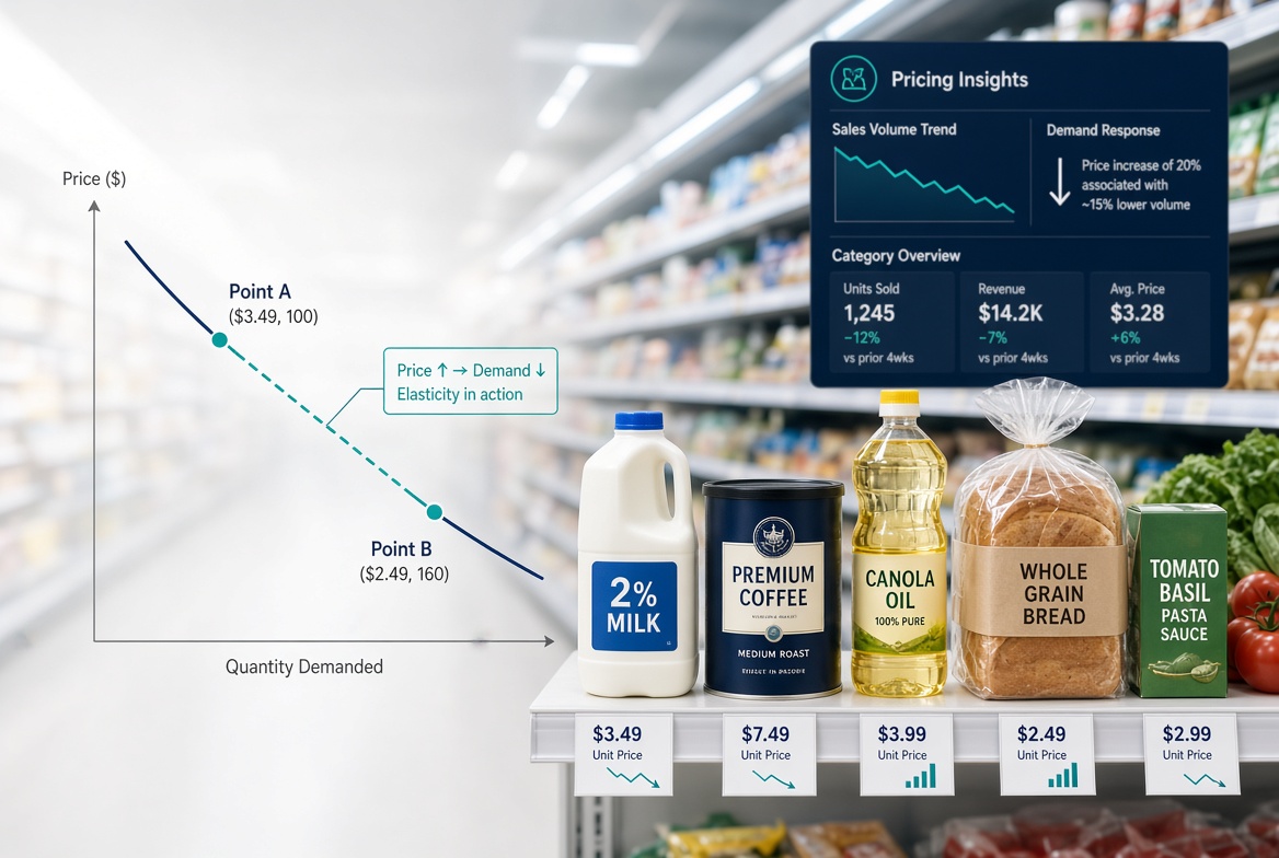
How Retailers Can Predict Customer Response to Price Changes

Introduction

A supermarket increases the price of a product by 5%.

What happens next?

Does demand fall by 2%?

5%?

10%?

Or does almost nothing happen?

The answer determines whether the price increase creates additional profit—or destroys revenue, customer traffic and margin.

This is the role of Price Elasticity of Demand.

In grocery retail, elasticity is particularly important because customers purchase thousands of products with very different levels of price sensitivity.

A 5% price increase on a premium specialty product may have almost no impact.

The same 5% increase on a highly visible staple such as milk, eggs, sugar or cooking oil may immediately affect customer behavior.

Therefore:

The right question is not “Can we increase the price?” but “How will customers respond if we do?”

Understanding Grocery Price Elasticity allows retailers to move from simple cost-based pricing toward data-driven price optimization.

1. What Is Price Elasticity?

Price Elasticity of Demand measures the percentage change in quantity demanded resulting from a percentage change in price.

The basic formula is:

Price Elasticity = % Change in Quantity Demanded ÷ % Change in Price

For example:

Price increases by:

10%

and unit sales decrease by:

20%

Then:

Elasticity = -20% ÷ 10% = -2.0

The negative sign reflects the normal inverse relationship between price and demand.

In retail discussions, the absolute value is often used:

Elasticity = 2.0

This means demand is highly responsive to price.

2. Elastic, Inelastic and Unit-Elastic Demand

There are three basic cases.

Elastic Demand

Absolute elasticity is greater than 1.

|E| > 1

A relatively small price change produces a larger percentage change in demand.

Example:

Price ↑ 5%
Volume ↓ 12%

This is elastic.

Inelastic Demand

Absolute elasticity is less than 1.

|E| < 1

Demand changes less than the price.

Example:

Price ↑ 5%
Volume ↓ 2%

This is inelastic.

Unit Elastic

Absolute elasticity equals 1.

|E| = 1

The percentage change in demand is approximately equal to the percentage change in price.

Example:

Price ↑ 5%
Volume ↓ 5%

3. Why Elasticity Matters So Much in Grocery Retail

Grocery retailers operate with thousands of products and relatively narrow margins in many categories.

A small pricing error can therefore have a significant financial impact.

Consider two products.

Product A

Price = $2.00

Price increase = 5%

New price = $2.10

Demand falls by 2%.

This product is relatively inelastic.

The retailer may increase revenue and potentially gross profit.

Product B

Price = $2.00

Price increase = 5%

Demand falls by 15%.

This product is highly elastic.

The price increase may reduce revenue and potentially damage profitability.

The same 5% price increase produced two completely different commercial outcomes.

That is why:

One pricing rule cannot work equally well across an entire grocery assortment.

4. Price Elasticity and Revenue

One of the most useful applications of elasticity is understanding the relationship between price and revenue.

Suppose:

Price = $10

Volume = 1,000 units

Revenue:

$10 × 1,000 = $10,000

Now increase price by 10%.

New price:

$11

If demand falls only 3%:

New volume:

970 units

New revenue:

$11 × 970 = $10,670

Revenue increases.

But suppose demand falls by 15%.

New volume:

850 units

New revenue:

$11 × 850 = $9,350

Revenue decreases.

Therefore:

The success of a price increase depends on the customer response—not simply the size of the increase.

5. Revenue Is Not the Same as Profit

This distinction is critical.

A retailer should not stop at:

Price × Volume = Revenue

The real objective is usually:

Gross Profit = (Selling Price − Variable Cost) × Volume

Consider:

Cost = $6

Current price = $10

Volume = 1,000

Gross profit:

($10 − $6) × 1,000 = $4,000

Now increase price to $11.

If volume falls to 850:

($11 − $6) × 850 = $4,250

Revenue falls from $10,000 to $9,350.

But gross profit increases from:

$4,000 → $4,250

This demonstrates why pricing decisions should be evaluated against profit, not revenue alone.

6. The Break-Even Volume Decline

A particularly useful managerial calculation is:

How much volume can we afford to lose before a price increase becomes unprofitable?

Suppose:

Current price = $10
Cost = $6
Current volume = 1,000

Current gross profit:

$4,000

New price:

$11

Contribution per unit:

To maintain the same gross profit:

$4,000 ÷ $5 = 800 units

Therefore, the retailer can lose:

200 units

or:

20% of volume

before gross profit falls below the original level.

This creates a practical pricing decision rule.

7. Elasticity Is Not the Same Across All Grocery Products

Different product characteristics produce different elasticity patterns.

Highly price-sensitive products may include:

Commodity-like products
Widely available branded products
Frequently purchased staples
Products with many substitutes
Products with transparent market prices

Less price-sensitive products may include:

Specialty products
Unique products
Premium products
Products with strong differentiation
Products with limited substitutes

But these are tendencies—not universal rules.

Actual elasticity must be measured from customer behavior.

8. The Connection Between KVI and Elasticity

This is where the previous article on KVI Identification becomes particularly important.

A product can be:

High KVI + High Elasticity

This is a strategically sensitive product.

Example:

Milk

If customers:

Know the price
Buy it frequently
Compare it with competitors
React strongly to price changes

then even a small price increase can damage price perception.

On the other hand:

Low KVI + Low Elasticity

may provide much more pricing flexibility.

This creates a useful pricing matrix.

	Low Elasticity	High Elasticity
Low KVI	Margin Opportunity	Monitor Carefully
High KVI	Strategic Pricing	Maximum Attention

The High KVI + High Elasticity quadrant deserves the strongest pricing discipline.

9. What Determines Grocery Price Elasticity?

Elasticity is influenced by multiple factors.

1. Availability of Substitutes

More substitutes generally mean greater price sensitivity.

2. Brand Strength

Strong brands may have lower elasticity among loyal customers.

3. Purchase Frequency

Frequently purchased products often receive more price attention.

4. Customer Income and Segment

Different customer segments may react differently to the same price change.

5. Product Necessity

Essential products can sometimes be less sensitive to price in the short term.

6. Competitive Price Gap

A large price gap can trigger switching.

7. Promotion Availability

Customers may delay purchases or switch products when promotions appear.

8. Pack Size

Customers may respond differently to a price increase versus a change in package size.

9. Seasonality

Demand sensitivity may change across seasons.

10. Shopping Mission

A customer doing a weekly stock-up may behave differently from a customer making an emergency purchase.

10. Cross-Price Elasticity

One of the most important concepts in grocery pricing is:

Cross-Price Elasticity.

This measures how demand for Product A changes when the price of Product B changes.

For example:

If Brand A increases its price, customers may switch to Brand B.

Then:

Brand A and Brand B are substitutes.

Consider:

Brand A = $3.00
Brand B = $2.80

If Brand A increases to $3.30 and Brand B sales increase significantly, there is evidence of substitution.

This is extremely important for category management.

A retailer should not analyze every SKU in isolation.

It should understand:

Product A ↔ Product B ↔ Product C

within the competitive category.

11. Example: Milk Category

Suppose a retailer has:

Product	Price	Units
Brand A	$2.00	5,000
Brand B	$2.10	3,500
Private Label	$1.80	2,000

Brand A increases its price to $2.20.

Total milk demand may remain relatively stable because some customers switch to:

Brand B
Private Label

Therefore, analyzing only Brand A’s elasticity may produce an incomplete answer.

The retailer needs to understand:

Category Elasticity + Cross Elasticity + Substitution

12. Category Elasticity vs. SKU Elasticity

This distinction is critical.

A SKU may be highly elastic.

But the overall category may be less elastic.

Why?

Because customers still need the category.

They simply switch brands.

For example:

If Brand A becomes expensive, customers may buy Brand B.

Therefore:

Brand A Volume ↓

but:

Total Category Volume → Stable

This means the retailer needs to distinguish:

SKU Demand

from:

Category Demand

and:

Store Demand.

13. Promotional Elasticity

Price elasticity also changes during promotions.

Suppose normal price is:

Promotion price:

Demand increases from:

1,000 → 1,400 units

The apparent elasticity may look extremely high.

But this does not necessarily mean the same elasticity will occur with a permanent price change.

Why?

Because promotions introduce additional factors:

Urgency
Visibility
Feature placement
Advertising
Stock-up behavior
Competitor response
Customer expectations

Therefore:

Promotional elasticity should not automatically be treated as permanent price elasticity.

14. The Stock-Up Effect

Grocery products can create unusual elasticity behavior because customers can stock up.

Suppose coffee normally sells for:

Promotion:

A customer who normally buys one package may buy:

2–3 packages

The retailer sees a dramatic increase in volume.

But some of the demand has simply been shifted from the future into the current period.

This is known as a stock-up effect.

Therefore, promotion analysis should examine:

Post-Promotion Demand

not just promotional-period sales.

15. Measuring Elasticity From Historical Data

A retailer can estimate elasticity using historical transaction data.

At minimum, the dataset should contain:

Date
SKU
Selling price
Units sold
Store
Promotion status
Competitor price
Stock availability
Season
Customer segment where available

Then the retailer can analyze periods where price changed while controlling for other factors.

A simple starting calculation is:

Elasticity = %ΔQuantity / %ΔPrice

But a mature model should go further.

16. Why Simple Elasticity Calculations Can Be Misleading

Suppose sales fell 20% after a 10% price increase.

It is tempting to conclude:

Elasticity = -2

But what if:

The competitor launched a promotion?
The product was out of stock?
The weather changed?
The product moved to a less visible shelf?
A new substitute entered the category?
The promotion ended?
The store lost traffic?

Then the observed sales decline cannot be attributed entirely to the price increase.

This is why serious elasticity analysis requires control variables.

17. A Better Elasticity Model

A more advanced model might consider:

Demand = f(Price, Competitor Price, Promotion, Seasonality, Availability, Store, Customer Segment, Trend)

Conceptually:

Q = f(P, Pc, Promo, Season, Availability, Store, Segment, Time)

This helps separate the impact of price from other demand drivers.

The objective is not merely to calculate a historical number.

It is to estimate:

What is likely to happen if we change the price?

18. The Importance of Competitor Prices

A customer’s response to your price depends partly on the price of alternatives.

Suppose your product is:

Competitor:

A price increase to:

$5.25

creates a meaningful price gap.

But if competitors simultaneously increase to:

$5.25

your relative position has not changed.

Therefore, grocery elasticity should often be analyzed using:

Relative Price

rather than absolute price alone.

A useful concept is:

Price Gap = Your Price − Competitor Price

or:

Price Index = Your Price ÷ Competitor Price × 100

19. Own-Price Elasticity vs. Competitive Elasticity

Retailers should distinguish:

Own-Price Elasticity

How demand changes when your price changes.

Cross-Price Elasticity

How demand changes when another product’s price changes.

Competitive Price Response

How your demand changes when competitor prices change.

These three dimensions together provide a much stronger view of pricing behavior.

20. Elasticity by Customer Segment

The same SKU can have different elasticity across customers.

For example:

Price-Sensitive Customer

Price ↑ 5%
Purchase probability ↓ significantly.

Loyal Customer

Price ↑ 5%
Purchase behavior changes very little.

Premium Customer

Price ↑ 5%
Almost no change.

This means:

Average Elasticity

may hide important differences.

If loyalty-card data is available, retailers can estimate elasticity by:

Customer segment
Geography
Store
Shopping mission
Frequency
Basket size

21. Store-Level Elasticity

Elasticity can also differ between stores.

For example:

A supermarket in a highly competitive urban location may have highly elastic demand.

A convenience store with limited nearby competition may have lower elasticity.

Therefore:

There may be no single elasticity number for a SKU across the entire retail network.

This has important implications for multi-store pricing.

22. Geographic Pricing

Consider the same product:

Store A

10 competitors within 2 km.

Store B

2 competitors within 10 km.

A uniform price may not be optimal.

Store A customers have more alternatives.

Store B customers have fewer immediate alternatives.

This does not automatically justify higher pricing at Store B, but it demonstrates why elasticity and competitive intensity can vary geographically.

23. Price Elasticity and Inventory

Inventory creates another important dimension.

Suppose a product is highly elastic.

Demand is weak.

Inventory is excessive.

The retailer may have a strong reason to reduce price.

But if inventory is low and the product is selling rapidly, a price reduction may simply accelerate stock depletion.

Therefore:

Price + Demand + Inventory

should be considered together.

This is one of the reasons modern pricing systems increasingly connect pricing with demand forecasting and inventory management.

24. Elasticity and Markdown Pricing

Markdowns are especially relevant for:

Short shelf-life products
Seasonal products
Fashion-related grocery/non-food products
Perishable items
Products approaching expiry

Suppose a product has:

Cost = $5

Regular price = $8

Remaining shelf life is short.

Reducing price to $6 may increase demand enough to recover more value than leaving the product at $8 and eventually writing it off.

The relevant question becomes:

What price maximizes recoverable margin before the product loses its economic value?

25. Elasticity and Dynamic Pricing

Dynamic pricing means adjusting prices based on changing market and demand conditions.

Potential inputs include:

Current demand
Forecast demand
Inventory
Competitor price
Seasonality
Time
Customer behavior
Product lifecycle

But dynamic pricing should not mean:

“Change prices constantly.”

That can damage customer trust.

The objective is:

Better price decisions at the right moments.

26. AI and Grocery Price Elasticity

AI can improve elasticity estimation by processing large volumes of transaction data.

It can identify relationships between:

Price
Volume
Competition
Promotions
Customer segments
Stores
Seasons
Inventory

AI can also estimate elasticity at multiple levels:

SKU

↓

Brand

↓

Category

↓

Store

↓

Customer Segment

This creates a much richer pricing model than a single elasticity coefficient.

27. Elasticity Scenario Simulation

One of the most useful applications is scenario modeling.

Suppose the retailer considers:

Price increase = 4%

The model can simulate:

Scenario A

Volume ↓ 2%

Scenario B

Volume ↓ 5%

Scenario C

Volume ↓ 8%

The retailer can then compare:

Revenue
Gross profit
Market position
Basket impact
Customer switching

This transforms pricing from:

“What do we think will happen?”

into:

“What happens under different demand assumptions?”

28. A Practical Elasticity Decision Matrix

KVI	Elasticity	Recommended Approach
High	High	Protect competitiveness
High	Low	Controlled price flexibility
Low	High	Test carefully
Low	Low	Greater margin opportunity

This is not a rigid rule.

It is a decision framework.

The retailer should combine it with:

Competition
Margin
Inventory
Basket impact
Customer segment
Strategic positioning

29. Common Elasticity Mistakes

Mistake 1: Assuming Every Product Has the Same Elasticity

It does not.

Mistake 2: Using Historical Elasticity Without Context

Historical demand may reflect promotions, stockouts or competitor actions.

Mistake 3: Ignoring Substitution

Customers may switch products rather than leave the category.

Mistake 4: Looking Only at Revenue

Profitability matters more than revenue alone.

Mistake 5: Ignoring Competitor Prices

Relative price often matters more than absolute price.

Mistake 6: Treating Promotional Response as Permanent Elasticity

Promotions create temporary behavioral effects.

Mistake 7: Using One Elasticity Number Across All Stores

Customer behavior can differ significantly by location.

30. Building a Grocery Elasticity Dashboard

A practical dashboard could include:

Demand

Units Sold
Sales Value
Volume Growth
Demand Trend

Price

Current Price
Previous Price
Price Change %
Competitor Price
Price Index

Elasticity

Own-Price Elasticity
Cross-Price Elasticity
Category Elasticity
Store-Level Elasticity

Profitability

Gross Margin %
Gross Margin Value
Contribution Margin

Customer

Switching Rate
Repeat Purchase
Basket Value
Customer Segment

Inventory

Stock Level
Days of Supply
Stockout Rate
Overstock

This dashboard connects the pricing decision to the wider commercial system.

31. Practical Example: Should We Raise the Price?

Suppose:

Current price = $4.00
Cost = $2.50
Volume = 10,000

Current gross profit:

($4.00 − $2.50) × 10,000 = $15,000

Management proposes:

Price = $4.20

The question is:

How much volume can we lose?

Contribution per unit becomes:

$4.20 − $2.50 = $1.70

Break-even volume:

$15,000 ÷ $1.70 = 8,824 units

Therefore, the retailer can lose approximately:

11.8% of volume

before gross profit falls below the original $15,000.

Now the retailer can compare this threshold with the estimated elasticity.

If expected volume decline is:

the increase may be attractive.

If expected decline is:

15%

the increase is probably unattractive.

This is a much stronger decision process than simply applying a target margin.

32. The Connection Between Elasticity and KVI Management

The previous article established:

KVI Identification

This article adds:

Elasticity

The next logical layer is:

Competitive Pricing

Together:

KVI + Elasticity + Competition

create the foundation for strategic grocery price management.

For example:

Product A

KVI Score = 95
Elasticity = -2.0
Competitor Gap = +7%

Recommended action:

High pricing attention

Product B

KVI Score = 25
Elasticity = -0.4
Competitor Gap = +4%

Recommended action:

Protect margin unless other factors justify intervention

This is how retailers move from simple pricing rules to differentiated pricing decisions.

33. From Elasticity to Price Optimization

Elasticity itself is not the final objective.

The objective is:

Optimal Price

A simplified optimization concept is:

Maximize Profit = (Price − Cost) × Demand(Price)

subject to:

Competitive constraints
Customer perception
Inventory
Pricing policies
Category architecture
Strategic positioning

This turns elasticity into a decision-making tool.

34. The Most Important Principle

Price elasticity should never be treated as a number sitting in a spreadsheet.

It is a representation of customer behavior under specific market conditions.

Elasticity changes when:

Competitors change prices
New substitutes appear
Promotions change
Customer income changes
Product availability changes
Seasons change
Consumer preferences change

Therefore:

Elasticity should be monitored, tested and updated—not calculated once and forgotten.

Conclusion

Grocery retail pricing becomes significantly more powerful when retailers understand not only what customers pay, but how customers respond when prices change.

Price Elasticity provides that missing link.

It helps answer questions such as:

Should we increase this price?
How much volume can we afford to lose?
Which products are highly price-sensitive?
Which products can support a margin increase?
Which KVIs require greater price protection?
How will customers substitute between brands?
How will competitor prices affect our demand?
Should the decision be made at SKU, category or store level?

The strongest pricing systems combine:

KVI Identification

Price Elasticity

Competitive Pricing

Promotion Analytics

Inventory Intelligence

Customer Behavior

Profit Optimization

The goal is not to predict customer behavior perfectly.

The goal is to make better pricing decisions with measurable evidence.

A retailer that understands elasticity can stop asking:

“What price should we charge?”

and start asking:

“What price creates the best balance between customer demand, competitive position and sustainable profit?”

That is the real purpose of Grocery Price Elasticity.

Practical Grocery Price Elasticity Framework

Collect Transaction Data

↓

Clean Price & Volume Data

↓

Identify Price Changes

↓

Control for Promotions & Stockouts

↓

Measure Own-Price Elasticity

↓

Analyze Cross-Price Elasticity

↓

Add Competitor Prices

↓

Segment by Store & Customer

↓

Simulate Price Scenarios

↓

Optimize for Profit

↓

Monitor Results

↓

Re-estimate Elasticity

This creates a continuous pricing learning loop:

Measure → Model → Simulate → Decide → Execute → Learn → Reprice

Related Articles

https://opexedg.com/post/grocery-retail-pricing-strategy/

https://opexedg.com/post/kvi-identification-grocery-retail/

https://opexedg.com/post/grocery-price-elasticity/

https://opexedg.com/post/competitive-pricing-grocery-retail/

https://opexedg.com/post/promotion-effectiveness-grocery-retail/

https://opexedg.com/post/ai-powered-retail-pricing/